GGU-PUMPTEST: Distance-time-drawdown method

The theoretical principles are described in Langguth/Voigt on pages 169 to 171. The example file "Distance-time-drawdown method.pvs" can be found in the program's example folder.

This method entails a drawdown in an extraction well with a constant pumping rate. At the same time, the course of the drawdown in this well is measured in at least two nearby monitoring wells.

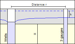
The graphical representation of the test results is in a semi-logarithmic scale (drawdown against "Time/square of distance [t/r²]"). The following data is required:

• distances (r) between the extraction well and the monitoring wells;
• the constant pumping rate in the extraction well;
• the aquifer thickness H;
• the specification of confined or unconfined aquifer;
• the drawdown h against time in the monitoring wells.

After defining the input values they are entered against t/r² (t = time, r = distance to monitoring well) and the best-fit curve determined.

Example:

This is the example for Gauges 3b, 11b and 6b in Langguth/Voigt. The principal boundary conditions correspond to those of the previous two examples.

In the menu item "File/New", press the "Distance-time-drawdown method" button and then go to the menu item "Edit/Edit values".

Using this method, you will see a dialog box in which you must first open the input box for the first individual test by clicking the "New" button. Enter the well name and the distance to the extraction well. Using the "Edit values" button, change the number of values to "24" and enter the measured data from Table 1.

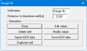
Repeat this procedure for the other two gauges, "6b" and "11b".

Gauge 6 b:

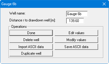
Using the "Edit values" button, change the number of values to "14" and enter the measured data from the following Table 3

Table 3 Gauge 6b measured data

Zeit [s]	h [m]
240.0	0.140
360.0	0.200
600.0	0.250
780.0	0.290
1140.0	0.350
1500.0	0.400
2040.0	0.450
2760.0	0.500
3900.0	0.550
4800.0	0.590
6450.0	0.650
8650.0	0.710
11450.0	0.760
13900.0	0.800

Gauge 11 b:

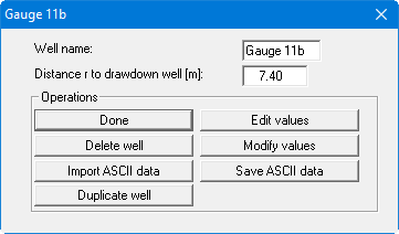
Using the "Edit values" button, change the number of values to "21" and enter the measured data from the following Table 4

Table 4 Gauge 11b measured data

Time [s]	h [m]
17.0	0.300
21.0	0.400
27.0	0.500
35.0	0.700
53.0	0.930
85.0	1.030
168.0	1.200
220.0	1.280
281.0	1.350
330.0	1.400
450.0	1.470
540.0	1.500
720.0	1.560
1080.0	1.640
1440.0	1.710
2100.0	1.790
3000.0	1.860
3900.0	1.900
5400.0	1.990
8300.0	2.070
14600.0	2.180

Go to the "Evaluation/Distance-time-drawdown method" menu item.

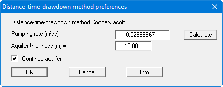
Enter the values in the dialog box and confirm with "OK".

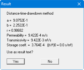
The "a" and "b" values describe the course of the best-fit curve through the data. The "r" value is the correlation coefficient, representing the quality of the best-fit curve. Below this, the permeability, the transmissivity and the storage coefficient are given. The (t/r²)0 value describes the intersection of the best-fit curve with the distance axis.

The solution given in Langguth/Voigt is:

• T = 8.9 · 10-3m²/s
• S = 4.6 · 10-4m²/s.

The minor differences are due to the purely visual evaluation employed by Langguth/Voigt.

If you adopt the result text, it is entered into the "Result text" box in the form .